Welcome to ipysensitivityprofiler’s documentation!

Jupyter Widgets for visualizing local sensitivities of callable Python functions in a notebook.

What is a sensitivity profile?

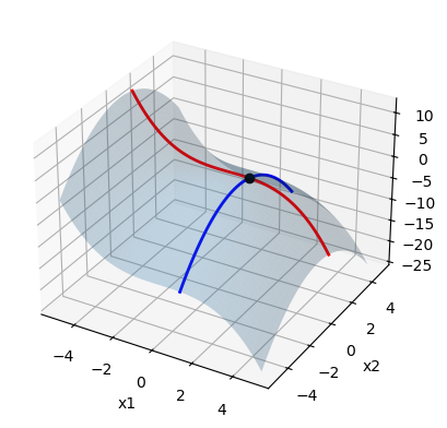
A local sensitivity profile is the trace of a function obtained by holding all dimensions fixed but one, as shown below. It can be thought of as the intersection of a cartesian plane (in which only one input is changing) and the response surface of interest.

show code

import numpy as np
import matplotlib.pyplot as plt
from mpl_toolkits.mplot3d import Axes3D


# Define equation
def f(x):
   return -0.1 * x[0] ** 3 - 0.5 * x[1] ** 2

# Point about which to evaluate sensitivities
x0 = np.array([[1], [1]])
y0 = f(x0)

# Define bounds of design space
lb = [-5, -5]  # x1_min, x2_min
ub = [ 5,  5]  # x1_max, x2_max

# Grid coordinates per dimension (for plotting response surface)
resolution = 100
x1 = np.linspace(lb[0], ub[0], resolution).reshape((1, -1))
x2 = np.linspace(lb[0], ub[0], resolution).reshape((1, -1))
X1, X2 = np.meshgrid(x1, x2)
x = np.concat([X1.reshape((1, -1)), X2.reshape((1, -1))])  # flatten grid
y = f(x)  # evaluate points
Y = y.reshape(X1.shape)  # reshape grid

# Plot response surface
fig = plt.figure()
ax = fig.add_subplot(111, projection='3d')
ax.plot_surface(X1, X2, Y, alpha=0.25)

# Plot profile along x1
x = np.concatenate([x1, x2])
x[1, :] = x0[1]
y = f(x)
ax.plot(x[0], x[1], y, alpha=1, color='red', linewidth=2)

# Plot profile along x2
x = np.concatenate([x1, x2])
x[0, :] = x0[0]
y = f(x)
ax.plot(x[0], x[1], y, alpha=1, color='blue', linewidth=2)

# Plot point about which sensitivities are evaluated
ax.plot(x0[0], x0[1], y0, "ko")
ax.set_xlabel("x1")
ax.set_ylabel("x2")
ax.set_zlabel("y")
plt.show()

Main Features

• Visualize multiple outputs against multiple inputs interactively

• Overlay more than one model at once

• Download pictures of individual plots (by clicking on the red dot)