1. Installation

The core algorithm is written in Python 3 and requires only numpy and orjson (for serialization):

pip install jenn

The matplotlib library is used to offer basic plotting utilities, such as checking goodness of fit or viewing sensitivity profiles, but it is entirely optional. To install:

pip install jenn[viz]

2. Data Structures

In order to use the library effectively, it is essential to understand its data structures. Mathematically, JENN is used to predict smooth, continuous functions of the form:

\[\boldsymbol{y} = f(\boldsymbol{x}) \qquad \Rightarrow \qquad \dfrac{\partial \boldsymbol{y}}{\partial \boldsymbol{x}} = f'(\boldsymbol{x})\]

where \(\frac{\partial \boldsymbol{y}}{\partial \boldsymbol{x}}\) is the Jacobian. For a single example, the associated quantities are given by:

\[\begin{split}\boldsymbol{x} = \left( \begin{matrix} x_1 \\ \vdots \\ x_{n_x} \end{matrix} \right) \in \mathbb{R}^{n_x} \quad \boldsymbol{y} = \left( \begin{matrix} y_1 \\ \vdots \\ y_{n_y} \end{matrix} \right) \in \mathbb{R}^{n_y} \quad \frac{\partial \boldsymbol{y}}{\partial \boldsymbol{x}} = \left( \begin{matrix} \frac{\partial y_1}{\partial x_1} & \dots & \frac{\partial y_1}{\partial x_{n_x}} \\ \vdots & \ddots & \vdots \\ \frac{\partial y_{n_y}}{\partial x_1} & \dots & \frac{\partial y_{n_y}}{\partial x_{n_x}} \\ \end{matrix} \right) \in \mathbb{R}^{n_y \times n_x}\end{split}\]

For multiple examples, denoted by \(m\), these quantities become vectorized as follows:

\[\begin{split}\boldsymbol{X} = \left( \begin{matrix} x_1^{(1)} & \dots & x_1^{(m)} \\ \vdots & \ddots & \vdots \\ x_{n_x}^{(1)} & \dots & x_{n_x}^{(m)} \\ \end{matrix} \right) \in \mathbb{R}^{n_x \times m} \qquad \boldsymbol{Y} = \left( \begin{matrix} y_1^{(1)} & \dots & y_1^{(m)} \\ \vdots & \ddots & \vdots \\ y_{n_y}^{(1)} & \dots & y_{n_y}^{(m)} \\ \end{matrix} \right) \in \mathbb{R}^{n_y \times m}\end{split}\]

Similarly, the vectorized version of the Jacobian becomes:

\[\begin{split}\boldsymbol{J} = \left( \begin{matrix} {\left( \begin{matrix} \frac{\partial y_1}{\partial x_1} & \dots & \frac{\partial y_1}{\partial x_{n_x}} \\ \vdots & \ddots & \vdots \\ \frac{\partial y_{n_y}}{\partial x_1} & \dots & \frac{\partial y_{n_y}}{\partial x_{n_x}} \\ \end{matrix} \right)}^{(1)} & \dots & {\left( \begin{matrix} \frac{\partial y_1}{\partial x_1} & \dots & \frac{\partial y_1}{\partial x_{n_x}} \\ \vdots & \ddots & \vdots \\ \frac{\partial y_{n_y}}{\partial x_1} & \dots & \frac{\partial y_{n_y}}{\partial x_{n_x}} \\ \end{matrix} \right)}^{(m)} \end{matrix} \right) \in \mathbb{R}^{n_y \times n_x \times m}\end{split}\]

Programmatically, these data structures are exclusively represented using shaped numpy arrays:

import numpy as np

# p = number of inputs
# K = number of outputs
# m = number of examples in dataset

x = np.array(
[
   [11, 12, 13, 14],
   [21, 22, 23, 24],
   [31, 32, 33, 34],
]
)  # array of shape (n_x, m) = (3, 4)

y = np.array(
[
   [11, 12, 13, 14],
   [21, 22, 23, 24],
]
)  # array of shape (n_y, m) = (2, 4)

dydx = np.array(
[
   [
      [111, 112, 113, 114],
      [121, 122, 123, 124],
      [131, 132, 133, 134],
   ],
   [
      [211, 212, 213, 214],
      [221, 222, 223, 224],
      [231, 232, 233, 234],
   ]
]
)  # array of shape (n_y, n_x, m) = (2, 3, 4)

p, m = x.shape
K, m = y.shape
K, p, m = dydx.shape

assert y.shape[0] == dydx.shape[0]
assert x.shape[0] == dydx.shape[1]
assert x.shape[-1] == y.shape[-1] == dydx.shape[-1]

3. Usage

This section provides a quick example to get started. Consider the task of fitting a simple 1D sinusoid using only three data points:

import numpy as np
import jenn

# Example function to be learned
f = lambda x: np.sin(x)
f_prime = lambda x: np.cos(x).reshape((1, 1, -1))  # note: jacobian adds a dimension

# Generate training data
x_train = np.linspace(-np.pi , np.pi, 3).reshape((1, -1))
y_train = f(x_train)
dydx_train = f_prime(x_train)

# Generate test data
x_test = np.linspace(-np.pi , np.pi, 30).reshape((1, -1))
y_test = f(x_test)
dydx_test = f_prime(x_test)

# Fit jacobian-enhanced neural net
genn = jenn.model.NeuralNet(
    layer_sizes=[x_train.shape[0], 3, 3, y_train.shape[0]],  # note: user defines hidden layer architecture
    ).fit(
        x_train, y_train, dydx_train, random_state=123  # see docstr for full list of hyperparameters
    )

# Fit regular neural net (for comparison)
nn = jenn.model.NeuralNet(
    layer_sizes=[x_train.shape[0], 3, 3, y_train.shape[0]]  # note: user defines hidden layer architecture
    ).fit(
        x_train, y_train, random_state=123  # see docstr for full list of hyperparameters
    )

# Predict response only
y_pred = genn.predict(x_test)

# Predict partials only
dydx_pred = genn.predict_partials(x_train)

# Predict response and partials in one step
y_pred, dydx_pred = genn.evaluate(x_test)

# Check how well model generalizes
assert jenn.utils.metrics.r_square(y_pred, y_test) > 0.99
assert jenn.utils.metrics.r_square(dydx_pred, dydx_test) > 0.99

Saving a model for later re-use:

genn.save("parameters.json")

Reloading the parameters a previously trained model:

new_model = jenn.model.NeuralNet(layer_sizes=[1, 12, 1]).load('parameters.json')

y_reloaded, dydx_reloaded = new_model.evaluate(x_test)

assert np.allclose(y_reloaded, y_pred)
assert np.allclose(dydx_reloaded, dydx_pred)

Optional plotting tools are available for convenience, provided matplotlib is installed:

from jenn.utils import plot

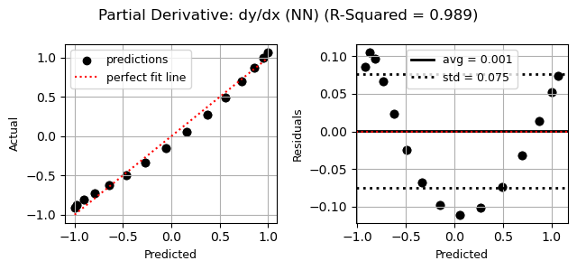
# Example: show goodness of fit of the partials
plot.goodness_of_fit(
    y_true=dydx_test[0],
    y_pred=genn.predict_partials(x_test)[0],
    title="Partial Derivative: dy/dx (NN)"
)

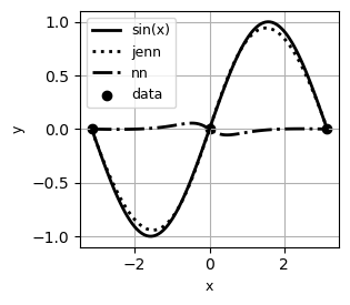
# Example: visualize local trends
plot.sensitivity_profiles(
    f=[f, genn.predict, nn.predict],
    x_min=x_train.min(),
    x_max=x_train.max(),
    x_true=x_train,
    y_true=y_train,
    resolution=100,
    legend=['sin(x)', 'jenn', 'nn'],
    xlabels=['x'],
    ylabels=['y'],
    show_cursor=False
)

4. Examples

Elaborated demo notebooks can be found on the project repo.