1. Installation

The library is written in Python 3 and available on PyPI:

pip install ipysensitivityprofiler

It renders in both Jupyter Lab and Jupyter Notebook. See the example notebooks in the project repo, or run them without installing anything on binder.

2. Example Usage

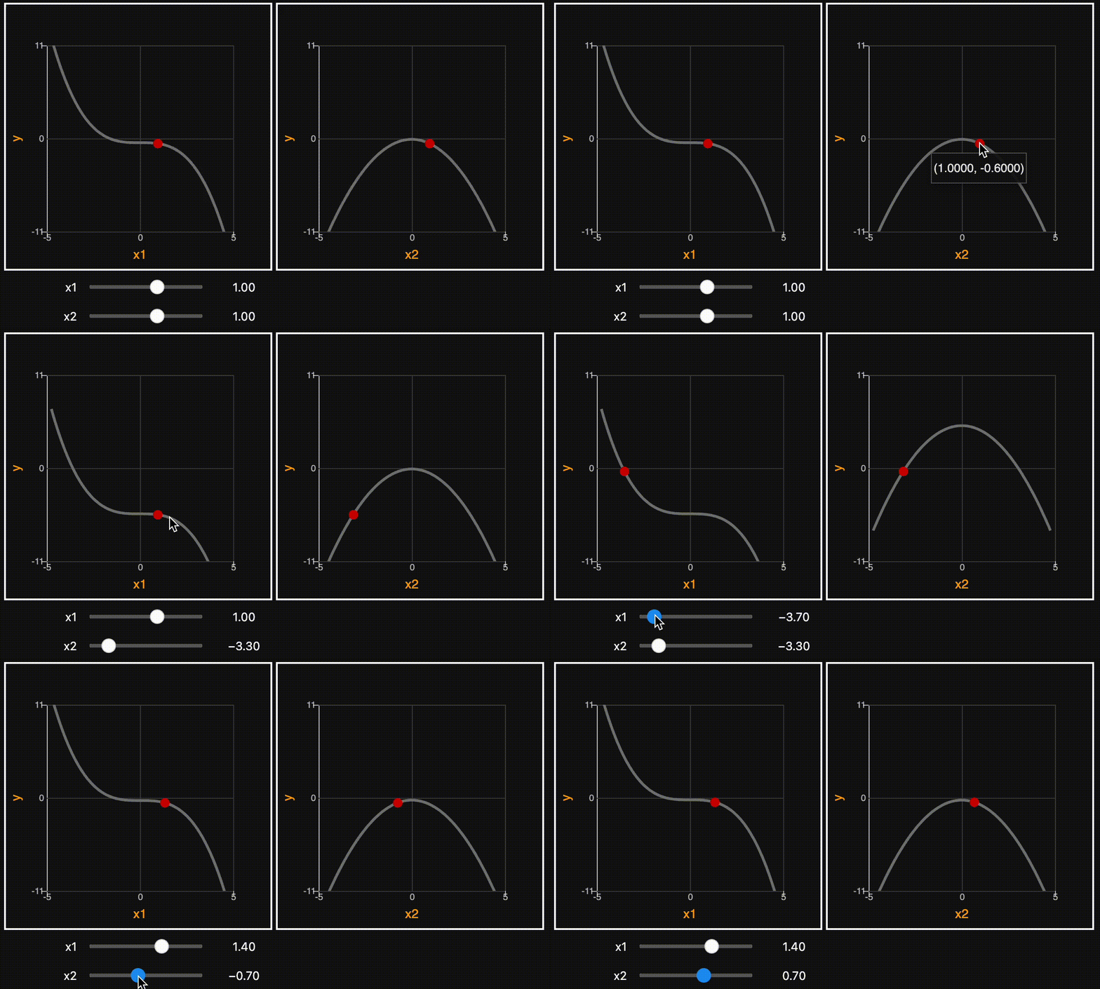
show code

import ipysensitivityprofiler as isp

def f(x):
   return -0.1 * x[:, 0] ** 3 - 0.5 * x[:, 1] ** 2

isp.profiler(
   models=[f],
   xmin=[-5, -5],
   xmax=[5, 5],
   ymin=[-10],
   ymax=[10],
   x0=[1, 1],
   resolution=100,
   xlabels=["x1", "x2"],
   ylabels=["y"],
)

3. Model Comparison

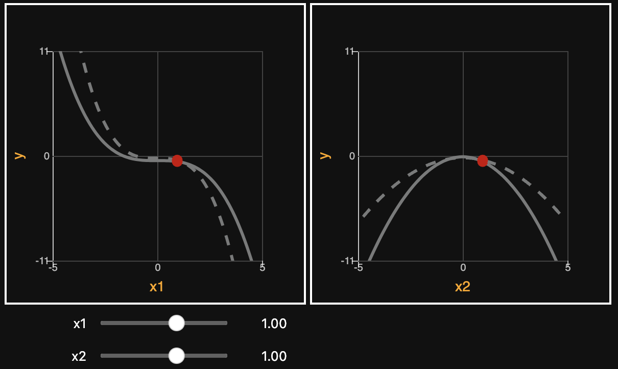
Taking advantage of the tool’s ability to render multiple models of the same thing on the same plot, two or more models can be compared against each other. Provided each model has the same signature, one can very quickly observe where they disagree:

show code

import ipysensitivityprofiler as isp

def f1(x):
   return -0.1 * x[:, 0] ** 3 - 0.5 * x[:, 1] ** 2

def f2(x):
   return -0.2 * x[:, 0] ** 3 - 0.25 * x[:, 1] ** 2

isp.profiler(
   models=[f1, f2],
   xmin=[-5, -5],
   xmax=[5, 5],
   ymin=[-10],
   ymax=[10],
   x0=[1, 1],
   resolution=100,
   xlabels=["x1", "x2"],
   ylabels=["y"],
)

4. Data Structures

The response \(f\) can be any callable Python function that maps \(\boldsymbol{x}\) to \(\boldsymbol{y}\), provided it is vectorized and adopts the following signature:

\[\boldsymbol{y} = f(\boldsymbol{x})\]

where \(\boldsymbol{x}\) and \(\boldsymbol{y}\) are multidimensional arrays defined below, in which \(n_x\) is the number of inputs, \(n_y\) is the number of outputs, and \(m\) is the number of examples:

\[\begin{split}\boldsymbol{x} = \left( \begin{matrix} x_1^{(1)} & \dots & x_{n_x}^{(1)} \\ \vdots & \ddots & \vdots \\ x_{1}^{(m)} & \dots & x_{n_x}^{(m)} \\ \end{matrix} \right) \in \mathbb{R}^{m \times n_x} \qquad \boldsymbol{y} = \left( \begin{matrix} y_1^{(1)} & \dots & y_{n_y}^{(1)} \\ \vdots & \ddots & \vdots \\ y_{1}^{(m)} & \dots & y_{n_y}^{(m)} \\ \end{matrix} \right) \in \mathbb{R}^{m \times n_y}\end{split}\]